Modelica® - A Unified Object-Oriented Language for Systems Modeling Language Specification Version 3.4 15 Stream Connectors 17 State Machines

Chapter 16 Synchronous Language Elements

This section presents language elements for describing synchronous behavior suited for implementation of control systems.

16.1 Introduction

16.1.1 Overview

[This chapter defines additional kinds of discrete-time variables and equations, as well as an additional kind of when-clause, in order to define sampled data systems in a safe way, so that the translator can provide good diagnostics in case of a modeling error.

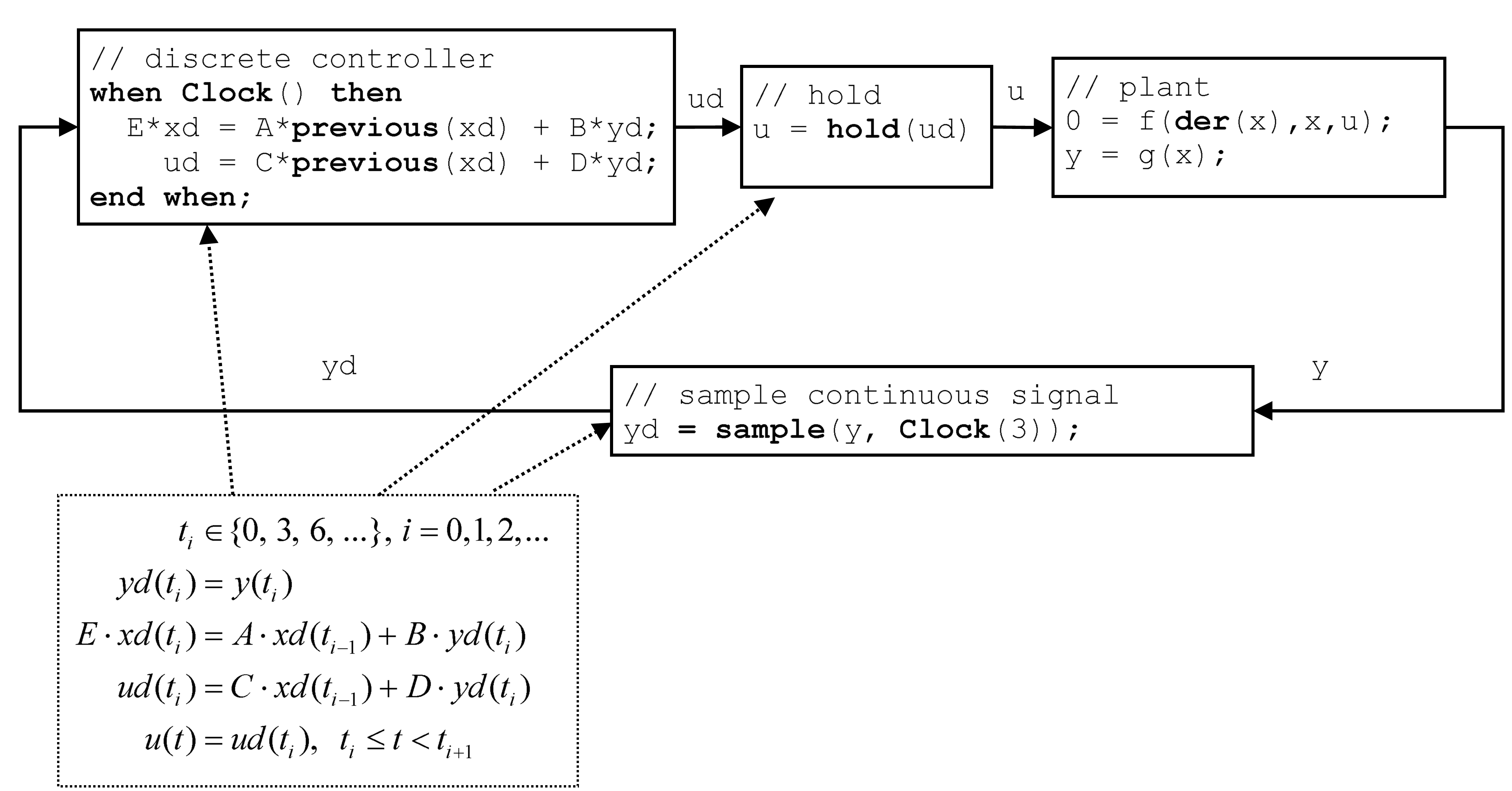
The following small example shows the most important elements

Figure 16.1: A continuous plant and a sampled data controller connected together with sample and (zero-order) hold elements

•

A periodic clock is defined with Clock(3). The argument of Clock(..) defines the sampling interval (for details see section 16.3).
•

Clocked variables (such as yd, xd, ud) are associated uniquely with a clock and can only be directly accessed when the associated clock is active. Since all variables in a clocked equation must belong to the same clock, clocking errors can be detected at compile time. If variables from different clocks shall be used in an equation, explicit cast operators must be used, such as sample(..) to convert from continuous-time to clocked discrete-time or hold(..) to convert from clocked discrete-time to continuous-time.
•

A continuous-time variable is sampled at a clock tick with the sample(..) operator. The operator returns the value of the continuous-time variable when the clock is active.
•

When no argument is defined for Clock(), the clock is deduced by clock inference.
•

For a when-clause with an associated clock, all equations inside the when-clause are clocked with the given clock. All equations on an associated clock are treated together and in the same way regardless of whether they are inside a when-clause or not. This means that automatic sampling and hold of variables inside the when-clause does not apply (explicit sampling and hold is required) and that general equations can be used in such when-clauses (this is not allowed for when-clauses with Boolean conditions, that require a variable reference on the left-hand side of an equation).
•

The when-clause in the controller could also be removed and the controller could just be defined by the equations:

⬇

  // discrete controller

  E*xd = A*previous(xd) + B*yd;

  ud = C*previous(xd) + D*yd;
•

The operator previous(xd) returns the value of xd at the previous clock tick. At the first sample instant, the start value of xd is returned.
•

A discrete-time signal (such as ud) is converted to a continuous-time signal with the hold(..) operator.
•

If a variable belongs to a particular clock, then all other equations where this variable is used, with the exception of as argument to certain special operators, belong also to this clock, as well as all variables that are used in these equations. This property is used for “clock inference” and allows to define an associated clock only at a few places (above only in the sampler, whereas in the discrete controller and the hold the sampling period is inferred)
•

The approach in this chapter is based on the clock calculus and inference system proposed by (Colaco and Pouzet 2003) and implemented in Lucid Synchrone version 2 and 3 (Pouzet 2006). However, the Modelica approach also uses multi-rate periodic clocks based on rational arithmetic introduced by (Forget et. al. 2008), as an extension of the Lucid Synchrone semantics. These approaches belong to the class of synchronous languages (Benveniste et. al. 2002).

16.1.2 Rationale for Clocked Semantics

Periodically sampled control systems could also be defined with standard when-clauses, see section 8.3.5, and the sample operator, see section 3.7.3. For example:

⬇

when sample(0,3) then

xd = A*pre(xd) + B*y;

u = C*pre(xd) + D*y;

end when;

Equations in a when-clause with a Boolean condition have the property that (a) variables on the left hand side of the equal sign are assigned a value when the when-condition becomes true and otherwise hold their value, (b) variables not assigned in the when-clause are directly accessed (= automatic “sample” semantics), and (c) the variables assigned in the when-clause can be directly accessed outside of the when-clause (= automatic “hold” semantics). This approach to define periodically sample data systems has the following drawbacks that are not present with the solution in this chapter using clocks and clocked equations:

1.

It is not possible to detect sampling errors due to the automatic sample and hold semantics. Examples:
1. a.
  
  If when-clauses in different blocks should belong to the same controller part, but by accident different when-conditions are given, then this is accepted (no error is detected)..
2. b.
  
  If a sampled data library such as the Modelica_LinearSystems2.Contoller library is used, at every block the sampling of the block has to be defined as integer multiple of a base sampling rate. If several blocks should belong to the same controller part, and different integer multiples are given, then the translator has to accept this (no error is detected).
2.

Due to the automatic sample and hold semantics, all variables assigned in a when-clause of the above kind must have an initial value because they might be used, before they are assigned a value the first time. As a result, all these variables are “discrete-time states” although in reality only a small subset of them need an initial value.
3.

Only a restricted form of equations can be used in a standard when-clause, since the left hand side has to be a variable, in order to identify the variables that are assigned in the when-clause. This is a severe restriction, especially if nonlinear control algorithms shall be defined. This restriction is not present for clocked equations.
4.

All equations belonging to a discrete controller must be in a when clause. If the controller is built-up with several building blocks, then the clock condition (sampling) must be explicitly propagated to all blocks. This is tedious and error prone. With clocked equations, the clock condition need to be defined only at one place, and otherwise is automatically propagated by clock inference.
5.

It is not possible to use a continuous-time model in when clauses (e.g. some advanced controllers use an inverse model of a plant in the feedforward path of the controller, see (Thümmel et. al. 2005)). This powerful feature of Modelica to use a nonlinear plant model in a controller would require to export the continuous-time model with an embedded integration method and then import it in an environment where the rest of the controller is defined. With clocked equations, clocked controllers with continuous-time models can be directly defined in Modelica.
6.

At a sample instant, an event iteration occurs (as for any other event). A clocked partition, as well as a when-clause with a sample(..) is evaluated exactly once at such an event instant. However, the continuous-time model to which the sampled data controller is connected, will be evaluated several times when the overall system is simulated. With when-clauses, the continuous-time part is typically evaluated three times at a sample instant (once, when the sample instant is reached, once to evaluate the continuous equations at the sample instant, and once when an event iteration occurs since a discrete variable v is changed and pre(v) appears in the equations). With clocked equations, no event iteration is triggered if a clocked variable v is changed and previous(v) appears in the equations, because the event iteration cannot change the value of v. As a result, typically the simulation model is evaluated twice at a sample instant and therefore the simulation is more efficient with clocked equations.

]

16.2 Definitions

In this section various terms are defined.

16.2.1 Clocks and Clocked Variables

In section 3.8.3 the term “discrete-time” Modelica expression and in section 3.8.4 the term “continuous-time” Modelica expression is defined. In this chapter, two additional kinds of discrete-time expressions/variables are defined that are associated to clocks and are therefore called “clocked discrete-time” expressions:

]

16.2.2 Base-Clock and Sub-Clock Partitions

The following concepts are used:

•

A “base-clock partition” identifies a set of equations and a set of variables which must be executed together in one task. Different base-clock partitions can be associated to separate tasks for asynchronous execution.
•

A “sub-clock partition” identifies a subset of equations and a subset of variables of a base-clock partition which are partially synchronized with other sub-clock partitions of the same base-clock partition, i.e., synchronized when the ticks of the respective clocks are simultaneous.

16.2.3 Argument Restrictions (Component Expression)

The built-in operators (with function syntax) defined in the following sections have partially restrictions on their input arguments that are not present for Modelica functions. To define the restrictions, the following term is defined:

: Component Expression:

A Component Reference which is an Expression, i.e. does not refer to models or blocks with equations. It is an instance of a (a) base type, (b) derived type, (c) record, (d) an array of such an instance (a-c), (e) one or more elements of such an array (d) defined by index expressions which are parameter expressions (see below), or (f) an element of records. [The essential features are that one or several values are associated with the instance, that start values can be defined on these values, and that no equations are associated with the instance. A Component Expression can be constant or can vary with time.]

In the following sections the following notation is partially used when defining the operators:

•

The input argument is a Component Expression:

The meaning is that the input argument when calling the operator must be a Component Expression.

[The reason for this restriction is that the start value of the input argument is returned before the first tick of the clock of the input argument and this is not possible for a general expression.

Examples:

⬇

  Real u1;

  Real u2[4];

  Complex c;

  Resistor R;

  ...

  y1 = previous(u1);    // fine

  y2 = previous(u2);    // fine

  y3 = previous(u2[2]); // fine

  y4 = previous(c.im);  // fine

  y5 = previous(2*u);   // error (general expression, no Component Expression)

  y6 = previous(R);     // error (component, no Component Expression)

]
•

The input argument is a parameter expression:

The meaning is that the input argument when calling the operator must have parameter variability, that is the argument must depend directly or indirectly only on parameters, constants or literals, see section 3.8.

[The reason for this restriction is that the value of the input argument needs to be evaluated during translation, in order that clock analysis can be performed during translation.

Examples:

⬇

  Real u;

  parameter Real p=3;

  ...

  y1 = subSample(u, factor=3);       // fine (literal)

  y2 = subSample(u, factor=2*p - 3); // fine (parameter expression)

  y3 = subSample(u, factor=3*u);     // error (general expression)

]
•

The input argument is an expression:

There is no restriction on the input argument when calling the operator. This notation is used to emphasis when a standard function call is used (“is an expression”), instead of restricting the input (“is a Component Expression”).

16.3 Clock Constructors

The following overloaded constructors are available to generate clocks:

Clock()

Inferred Clock

The operator returns a clock that is inferred. [Example:

⬇

when Clock() then // equations are on the same clock

x = A*previous(x) + B*u;

Modelica.Utilities.Streams.print

("clock ticks at = " + String(sample(time)));

end when;

Note, in most cases, the operator is not needed and equations could be written without a when-clause (but not in the example above, since the “print” statement is otherwise not associated to a clock). This style is useful if a modeler would clearly like to mark the equations that must belong to one clock (although a tool could figure this out as well, if the when-clause is not present).]

Clock(intervalCounter,resolution)

Clock with Rational Interval

The first input argument, intervalCounter, is a clocked Component Expression (see section 16.2.3) or a parameter expression of type Integer with min=0. The optional second argument resolution (default=1) is a parameter expression of type Integer with min=1 and unit “Hz”. If intervalCounter is a parameter expression with value zero, the period of the clock is derived by clock inference, see section 16.7.5. The output argument is of base type Clock that ticks when time becomes t_start, t_start+interval1, t_start+interval1+interval2, … The clock starts at the start of the simulation t_start or when the controller is switched on. At the start of the simulation, previous(intervalCounter) = intervalCounter.start and the clocks ticks the first time. At the first clock tick intervalCounter must be computed and the second clock tick is then triggered at interval1=intervalCounter/resolution. At the second clock tick at time tstart+interval1, a new value for intervalCounter must be computed and the next clock tick is scheduled at interval2 = intervalCounter/resolution, and so on. If interval is a parameter expression, the clock defines a periodic clock. [The given interval and time shift can be modified by using the subSample, superSample, shiftSample and backSample operators on the returned clock, see section 16.5.2. Example:

⬇

// first clock tick: previous(nextInterval)=2

Integer nextInterval(start=2);

Real y1(start=0);

Real y2(start=0);

equation

when Clock(2,1000) then

// periodic clock that ticks at 0, 0.002, 0.004, …

y1 = previous(y1) + 1;

end when;

when Clock(nextInterval, 1000) then

// interval clock that ticks at 0, 0.003, 0.007, 0.012, …

nextInterval = previous(nextInterval) + 1;

y2 = previous(y2) + 1;

end when;

] Note that operator interval(c) of Clock c = Clock(nextInterval,resolution) returns:previous(intervalCounter)/resolution; // in seconds

Clock(interval)

Clock with Real Interval

The input argument, interval, is a clocked Component Expression (see section 16.2.3) or a parameter expression of type Real with min=0.0 and unit “s”. The output argument is of base type Clock that ticks when time becomes t_start, t_start+interval1, t_start+interval1+interval2, … The clock starts at the start of the simulation t_start or when the controller is switched on. Here the next clock tick is scheduled at interval1 = previous(interval) = interval.start. At the second clock tick at time t_start+interval1, the next clock tick is scheduled at interval2 = previous(interval), and so on. If interval is a parameter expression, the clock defines a periodic clock. [Note, the clock is defined with previous(interval). Therefore, for sorting the input argument is treated as known. The given interval and time shift can be modified by using the subSample, superSample, shiftSample and backSample operators on the returned clock, see section 16.5.2. There are restrictions where this operator can be used, see Clock expressions below.]

Clock(condition,startInterval)

Clock with Boolean Condition

The input argument, condition, is a continuous-time expression of type Boolean. The optional startInterval argument (default = 0.0) is the value returned by the operator interval() at the first tick of the clock, see section 16.9. The output argument is of base type Clock that ticks when edge(condition) becomes true. [This clock is used to trigger a clocked partition due to a state event, that is a zero-crossing of a Real variable, in a continuous-time partition or due to a hardware interrupt that is modeled as Boolean in the simulation model. Example:

⬇

Clock c = Clock(angle > 0, 0.1) // before first tick of c:

// interval(c) = 0.1

The implicitly given interval and time shift can be modified by using the subsample, superSample, shiftSample and backSample operators on the returned clock, see section 16.5.2, provided the base interval is not smaller than the implicitly given interval. ]

Clock(c,solverMethod)

Solver Clock

The first input argument “c” is a clock and the operator returns this clock. The returned clock is associated with the second input argument of type String “solverMethod”. The meaning of solverMethod is defined in section 16.8.2. If the second input argument solverMethod is an empty String, then no integrator is associated with the returned clock. [Examples:

⬇

Clock c1 = Clock(1,10) // 100 ms, no solver

Clock c2 = Clock(c1, "ImplicitTrapezoid");

// 100 ms, ImplicitTrapezoid solver

Clock c3 = Clock(c2, ""); // 100 ms, no solver

]

Besides inferred clocks and solver clocks, one of the following mutually exclusive associations of clocks are possible in one base partition:

1.

One or more Rational interval clocks, provided they are consistent with each other, see section 16.7.5.
[For example, assume “y = subSample(u)”, and Clock(1,10) is associated to “u” and Clock(2,10) is associated with “y”, then this is correct, but it would be an error if “y” is associated to a Clock (1,3). ]
2.

Exactly one Real interval clock. [Assume“Clock c = Clock(2.5)”, then variables in the same base partition can be associated multiple times with “c” but not multiple times with “Clock(2.5)”]
3.

Exactly one Boolean clock.
4.

A default clock, if neither a Real interval, nor a Rational interval nor a Boolean clock is associated with a base partition. In this case the default clock is associated with the fastest sub-clock partition. [Typically, a tool will use Clock(1.0) as a default clock and will raise a warning, that it selected a default clock.]

Clock variables can be used in a restricted form of expressions. Generally, every expression containing clock variables must have parametric variability [in order that clock analysis can be performed when translating a model.]. Otherwise, the following expressions are allowed:

•

Declaring arrays of clocks [Example: Clock c1[3] ={Clock(1), Clock(2), Clock(3)} ]
•

Array constructors of clocks: {}, [], cat(...).
•

Array access of clocks [Example: sample(u, c1[2])]
•

Equality of clocks [Example: c1 = c2].
•

If-expressions of clocks in equations
[Example: Clock c2 = if f>0 then subSample(c1, f) elseif f<0 then superSample(c1, f) else c1].
•

Clock variables can be declared in models, blocks, connectors, and records,. A Clock variable can be declared with the prefixes input, output, inner, outer, but not with the prefixes flow, stream, discrete, parameter, or constant [Example: connector ClockInput = input Clock;]

16.4 Discrete States

The previous value of a clocked variable can be accessed with the previous operator. Such a variable is called a clocked state variable.

previous(u)

The input argument is a Component Expression (see section 16.2.3) or a parameter expression. The return argument has the same type as the input argument. Input and return arguments are on the same clock. At the first tick of the clock of u or after a reset transition (see section 17.3.2), the start value of u is returned, see section 16.9. At subsequent activations of the clock of u, the value of u from the previous clock activation is returned.

16.5 Partitioning Operators

A set of “clock conversion operators” together act as boundaries between different clock partitions.

16.5.1 Base-clock conversion operators

The following operators convert between a continuous-time and a clocked-time representation and vice versa:

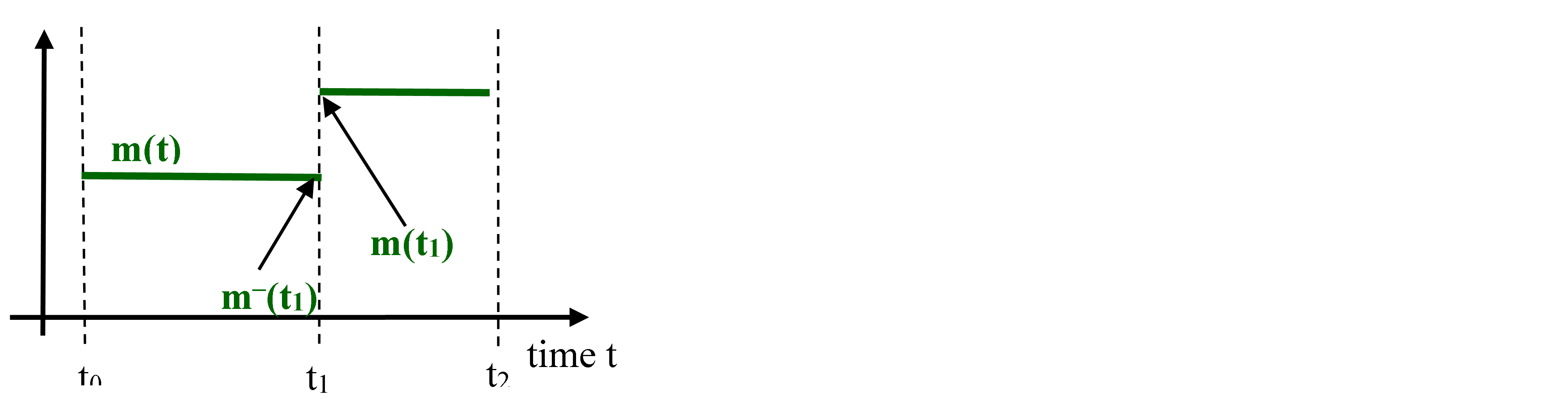
sample(u, c)

Input argument u is a continuous-time expression according to section 3.8.4. The optional input argument c is of type Clock. The operator returns a clocked variable that has c as associated clock and has the value of the left limit of u when c is active (that is the value of u just before the event of c is triggered). If argument c is not provided, it is inferred, see section 16.7.5. [Since the operator returns the left limit of u, it introduces an infinitesimal small delay between the continuous-time and the clocked partition. This corresponds to the reality, where a sampled data system cannot act infinitely fast and even for a very idealized simulation, an infinitesimal small delay is present. The consequences for the sorting are discussed below. Input argument u can be a general expression, because the argument is continuous-time and therefore has always a value. It can also be a constant, a parameter or a piecewise constant expression. Note that sample() is an overloaded function: If sample(..) has two input arguments and the second argument is of type Real, it is the operator from section 3.7.3. If sample(..) has one input argument, or it has two input arguments and the second argument if of type Clock, it is the base-clock conversion operator from this section.]

hold(u)

Input argument u is a clocked Component Expression (see section 16.2.3) or a parameter expression. The operator returns a piecewise constant signal of the same type of u. When the clock of u ticks, the operator returns u and otherwise returns the value of u from the last clock activation. Before the first clock activation of u, the operator returns the start value of u, see section 16.9. [Since the input argument is not defined before the first tick of the clock of u, the restriction is present, that it must be a Component Expression (or a parameter expression), in order that the initial value of u can be used in such a case.]

[Example:

Assume there is the following model:

⬇

Real y(start=1), yc;

equation

der(y) + y = 2;

yc = sample (y, Clock(0.1));

initial equation

der(y) = 0;

The value of yc at the first clock tick is yc=2 (and not yc=1 ). The reason is that the continuous-time model der(y)+y=2 is first initialized and after initialization y has the value 2. At the first clock tick at time=0, the left limit of y is 2 and therefore yc = 2.

Sorting of a simulation model:
Since sample(u) returns the left limit of u, and the left limit of u is a known value, all inputs to a base-clock partition are treated as known during sorting. Since a periodic and interval clock can tick at most once at a time instant, and since the left limit of a variable does not change during event iteration (i.e., re-evaluating a base-clock partition associated with a condition clock always gives the same result because the sample(u) inputs do not change and therefore need not to be re-evaluated) all base-clock partitions, see section 16.7.3, need not to be sorted with respect to each other. Instead, at an event instant, active base-clock partitions can be evaluated first (and once) in any order. Afterwards, the continuous-time partition is evaluated. Event iteration takes place only over the continuous-time partition. In such a scenario, accessing the left limit of u in sample(u) just means to pick the latest available value of u when the partition is entered, storing it in a local variable of the partition and only using this local copy during evaluation of the equations in this partition.]

16.5.2 Sub-clock conversion operators

The following operators convert between synchronous clocks:

The operators in this table have the following properties: The input argument u is a clocked expression or an expression of type Clock. [The operators can operate on all types of clocks]. If u is a clocked expression, the operator returns a clocked variable that has the same type as the expression. If u is an expression of type Clock, the operator returns a Clock. The optional input arguments factor (default=0, min=0), and resolution (default=1, min=1) are parameter expressions of type Integer. The input arguments shiftCounter and backCounter are parameter expressions of type Integer (min=0).

subSample(u, factor)

The clock of y = subSample(u,factor) is factor-times slower than the clock of u. At every factor ticks of the clock of u, the operator returns the value of u.. The first activation of the clock of y coincides with the first activation of the clock of u. If argument factor is not provided or is equal to zero, it is inferred, see section 16.7.5.

superSample(u, factor)

The clock of y = superSample(u,factor) is factor-times faster than the clock of u. At every tick of the clock of y, the operator returns the value of u from the last tick of the clock of u. The first activation of the clock of y coincides with the first activation of the clock of u. If argument factor is not provided or is equal to zero, it is inferred, see section 16.7.5. If a Boolean clock is associated to a base-clock partition, all its sub-clock partitions must have resulting clocks that are sub-sampled with an Integer factor with respect to this base clock. [Example:

⬇

Clock u = Clock(x > 0);

Clock y1 = subSample(u,4);

Clock y2 = superSample(y1,2); // fine; y2 = subSample(u,2)

Clock y3 = superSample(u ,2); // error

Clock y4 = superSample(y1,5); // error

]

shiftSample(u,

shiftCounter, resolution)

[The first activation of the clock of y = shiftSample(..) is shifted in time shiftCounter/resolution*interval(u) later than the first activation of the clock of u.]. Conceptually, the operator constructs a clock “cBase”

⬇

Clock cBase = subSample(superSample(u,resolution), shiftCounter)

and the clock of y = shiftSample(..) starts at the second clock tick of cBase. At every tick of the clock of y, the operator returns the value of u from the last tick of the clock of u. [Note, due to the restriction of superSample on Boolean clocks, shiftSample can only shift the number of ticks of the Boolean clock, but cannot introduce new ticks. Example:

⬇

// Rational interval clock

Clock u = Clock(3, 10); // ticks: 0, 3/10, 6/10, ..

Clock y1 = shiftSample(u,1,3); // ticks: 1/10, 4/10,

...

// Boolean clock

Clock u = Clock(sin(2*pi*time)>0, startInterval=0.0)

// ticks: 0.0, 1.0, 2.0, 3.0, …

Clock y1 = shiftSample(u,2); // ticks: 2.0, 3.0, …

Clock y2 = shiftSample(u,2,3);// error (resolution must be 1)

]

backSample(u,

backCounter, resolution)

The input argument u is either a Component Expression (see section 16.2.3) or an expression of type Clock. [The first activation of the clock of y = backSample(..) is shifted in time backCounter/resolution*interval(u) before the first activation of the clock of u]. Conceptually, the operator constructs a clock “cBase”

⬇

Clock cBase = subSample(superSample(u,resolution), backCounter)

and the clock of y = shiftSample(..) is shifted a time duration before the clock of u, such that this duration is identical to the duration between the first and second clock tick of cBase. It is an error, if the clock of y starts before the base clock of u. At every tick of the clock of y, the operator returns the value of u from the last tick of the clock of u. If u is a clocked Component Expression, the operator returns the start value of u, see section 16.9, before the first tick of the clock of u. [Example:

⬇

// Rational interval clock 1

Clock u = Clock(3, 10); // ticks: 0, 3/10, 6/10, ..

Clock y1 = shiftSample(u,3); // ticks: 9/10, 12/10, ..

Clock y2 = backSample(y1,2); // ticks: 3/10, 6/10,

...

Clock y3 = backSample(y1,4); // error (ticks before u)

Clock y4 = shiftSample(u,2,3); // ticks: 2/10, 5/10,

...

Clock y5 = backSample(y4,1,3); // ticks: 1/10, 4/10,

...

// Boolean clock

Clock u = Clock(sin(2*pi*time) > 0, startInterval=xx)

// ticks: 0, 1.0, 2.0, 3.0, ….

Clock y1 = shiftSample(u,3); // ticks: 3.0, 4.0, …

Clock y2 = backSample(y1,2); // ticks: 1.0, 2.0, …

]

noClock(u)

The clock of y = noClock(u) is always inferred. At every tick of the clock of y, the operator returns the value of u from the last tick of the clock of u. If noClock(u) is called before the first tick of the clock of u, the start value of u is returned.

[Clarification of backSample(..) operator:

Let a and b be positive integers with a < b, and

⬇

yb = backSample (u, a , b)

ys = shiftSample(u, b-a, b)

Then when ys exists, also yb exists and ys = yb.
The variable yb exists for the above parameterization with a<b one clock tick before ys. Therefore, backSample is basically a shiftSample with a different parameterization and the clock of backSample.y ticks before the clock of u. Before the clock of u ticks, yb = u.start.

Clarification of noClock(..) operator:

Note, that noClock(u) is not equivalent to sample(hold(u)). Consider the following model:

⬇

model NoClockVsSampleHold

Clock clk1 = Clock(0.1);

Clock clk2 = subSample(clk1,2);

Real x(start=0), y(start=0), z(start=0);

equation

when clk1 then

x = previous (x) + 0.1;

end when;

when clk2 then

y = noClock (x); // most recent value of x

z = sample (hold(x)); // left limit of x (infinitesimally delayed)!

end when;

end NoClockVsSampleHold;

Due to the infinitesimal delay of sample; z will not show the current value of x as clk2 ticks, but will show its previous value (left limit). However, y will show the current value, since it has no infinitesimal delay.]

16.6 Clocked When Clause

In addition to the previously discussed conditional when-clause, a clocked when-clause is introduced:

⬇

when clock-expression then

clocked-equation

...

end when;

The clocked when-clause cannot be nested and does not have any elsewhen part. It cannot be used inside an algorithm. General equations are allowed in a clocked when-clause.

For a clocked when-clause, all equations inside the when-clause are clocked with the same clock given by the clock-expression.

16.7 Clock Partitioning

This section defines how clock-partitions and clocks associated with equations are inferred. [Typically clock partitioning is performed before sorting the equations. The benefit is that clocking and symbolic transformation errors are separated.]

Every clocked variable is uniquely associated with exactly one clock.

After model flattening, every equation in an equation section, every expression and every algorithm section is either continuous-time, or it is uniquely associated with exactly one clock. In the latter case it is called a clocked equation, a clocked expression or clocked algorithm section respectively. The associated clock is either explicitly defined by a when-clause, see section 16.5.2, or it is implicitly defined by the requirement that a clocked equation, a clocked expression and a clocked algorithm section must have the same clock as the variables used in them with exception of the expressions used as first arguments in the conversion operators of section 16.5. Clock inference means to infer the clock of a variable, an equation, an expression or an algorithm section if the clock is not explicitly defined and is deduced from the required properties in the previous two paragraphs.

All variables in an expression without clock conversion operators must have the same clock to infer the clocks for each variable and expression. The clock inference works both forward and backwards regarding the data flow and is also being able to handle algebraic loops. The clock inference method uses the set of variable incidences of the equations, i.e., what variables that appear in each equation.

Note that incidences of the first argument of clock conversion operators of section 16.5 are handled specially.

16.7.1 Flattening of Model

The clock partitioning is conceptually performed after model flattening, i.e., redeclarations have been elaborated, arrays of model components expanded into scalar model components, and overloading resolved. Furthermore, function calls to inline functions have been inlined. [This is called “conceptually”, because a tool might do this more efficiently in a different way, provided the result is the same as if everything is flattened. For example, array and matrix equations and records don’t not need to be expanded if they have the same clock.]

Furthermore, each non-trivial expression (non-literal, non-constant, non-parameter, non-variable), expr_i, appearing as first argument of any clock conversion operator is recursively replaced by a unique variable, v_i, and the equation v_i = expr_i is added to the equation set.

16.7.2 Connected Components of the Equations and Variables Graph

Consider the set E of equations and the set V of unknown variables (not constants and parameters) in a flattened model, i.e. M = <E, V>. The partitioning is described in terms of an undirected graph <N, F> with the nodes N being the set of equations and variables, N = E + V. The set incidence(e) for an equation e in E is a subset of V, in general, the unknowns which lexically appear in e. There is an edge in F of the graph between an equation, e, and a variable, v, if v = incidence(e):

F=\{(e,v):e\in E,v\in\text{incidence}(e)\}

A set of clock partitions is the “connected components” (Wikipedia, “Connected components”) of this graph with appropriate definition of the incidence operator.

16.7.3 Base-clock Partitioning

The goal is to identify all clocked equations and variables that should be executed together in the same task, as well as to identify the continuous-time partition.

The base-clock partitioning is performed with base-clock inference which uses the following incidence definition:

incidence(e) = the unknown variables, as well as variables x in der(x), pre(x), and previous(x),
	which lexically appear in e
		except as first argument of base-clock conversion operators: sample() and hold().

The resulting set of connected components, is the partitioning of the equations and variables, B_i = <E_i, V_i>, according to base-clocks and continuous-time partitions.

The base clock partitions are identified as clocked or as continuous-time partitions according to the following properties:

A variable u in sample(u) and a variable y in y = hold(ud) is in a continuous-time partition.

Correspondingly, variables u and y in y = sample(uc), y = subSample(u), y = superSample(u), y = shiftSample(u), y = backSample(u), y = previous(u), are in a clocked partition. Equations in a clocked when clause are also in a clocked partition. Other partitions where none of the variables in the partition are associated with any of the operators above have an unspecified partition kind and are considered continuous-time partitions.

All continuous-time partitions are collected together and form “the” continuous-time partition.

[Example:

⬇

// Controller 1

ud1 = sample(y,c1);

0 = f1(yd1, ud1, previous(yd1));

// Controller 2

ud2 = superSample(yd1,2);

0 = f2(yd2, ud2);

// Continuous-time system

u = hold(yd2);

0 = f3(der(x1), x1, u);

0 = f4(der(x2), x2, x1);

0 = f5(der(x3), x3);

0 = f6(y, x1, u);

After base clock partitioning, the following partitions are identified:

⬇

// Base partition 1 // clocked partition

ud1 = sample (y,c1); // incidence(e) = {ud1}

0 = f1(yd1, ud1, previous(ud1)); // incidence(e) = {yd1,ud1}

ud2 = superSample (yd1,2); // incidence(e) = {ud2, yd1}

0 = f2(yd2, ud2); // incidence(e) = {yd2, ud2}

// Base partition 2 // continuous-time partition

u = hold (yd2); // incidence(e) = {u}

0 = f3(der(x1), x1, u); // incidence(e) = {x1,u}

0 = f4(der(x2), x2, x1); // incidence(e) = {x2,x1}

0 = f6(y, x1, u); // incidence(e) = {y,x1,u}

// Identified as separate partition, but belonging to partition 2

0 = f5(der(x3), x3); // incidence(e) = {x3}

]

16.7.4 Sub-clock Partitioning

For each clocked partition B_i, identified in section 16.7.3, the sub-clock partitioning is performed with sub-clock inference which uses the following incidence definition:

incidence(e) = the unknown variables, as well as variables x in der(x), pre(x), and previous(x),
	which lexically appear in e
		except as first argument of sub-clock conversion operators:
			subSample, superSample, shiftSample, backSample, and noClock.

The resulting set of connected components, is the partitioning of the equations and variables, S_ij = <E_ij, V_ij>, according to sub-clocks.

It can be noted that:

$E_{ij}\bigcap E_{kl}=\emptyset~{}\forall i\neq{}k,j\neq{}l$

$V_{ij}\bigcap V_{kl}=\emptyset~{}\forall i\neq{}k,j\neq{}l$

$V=\bigcup V_{ij}$

$E=\bigcup E_{ij}$

[Example:

After sub-clock partitioning of the example from section 16.7.3, the following partitions are identified:

⬇

// Base partition 1 (clocked partition)

// Sub-clock partition 1.1

ud1 = sample (y,c1); // incidence(e) = {ud1}

0 = f1(yd1,ud1,previous(yd1)); // incidence(e) = {yd1,ud1}

// Sub-Clock partition 1.2

ud2 = superSample (yd1,2); // incidence(e) = {ud2}

0 = f2(yd2,ud2); // incidence(e) = {yd2,ud2}

// Base partition 2 (no sub-clock partitioning, since continuous-time)

u = hold (yd2);

0 = f3(der(x1), x1, u);

0 = f4(der(x2), x2, x1);

0 = f5(der(x3), x3);

0 = f6(y, x1, u);

]

16.7.5 Sub-clock Inferencing

For each base-clock partition, the base interval needs to be determined and for each sub-clock partition, the sub-sampling factors and shift need to be determined. For each sub-clock partition, the interval might be rational or Real type and known or parametric or being unspecified. The sub-clock partition intervals are constrained by subSample and superSample factors which might be known (or parametric) or unspecified and by shiftSample shiftCounter and resolution or backSample, backCounter and resolution. This constraint set is used to solve for all intervals and sub-sampling factors and shift of the sub-clock partitions. The model is erroneous if no solution exist.

[It must be possible to determine that the constraint set is valid at compile time. However, in certain cases, it could be possible to defer providing actual numbers until run-time. ]

It is required that accumulated sub- and super sampling factors in the range of 1 to 2⁶³ can be handled.

[64 bit internal representation of numerator and denominator with sign can be used and gives
minimum resolution 1.08E-19 seconds and maximum range 9.22E+18 seconds = 2.92E+11 years.]

16.8 Continuous-Time Equations in Clocked Partitions

[The goal is that every continuous-time Modelica model can be utilized in a sampled data control system. This is achieved by solving the continuous-time equations with a defined integration method between clock ticks. With this feature, it is for example possible to invert the nonlinear dynamic model of a plant, see (Thümmel et.al. 2005), and use it in a feedforward path of an advanced control system that is associated with a clock.

This feature also allows to define multi-rate systems: Different parts of the continuous-time model are associated to different clocks and are solved with different integration methods between clock ticks, e.g., a very fast sub-system with an implicit solver with a small step-size and a slow sub-system with an explicit solver with a large step-size.]

With the language elements defined in this section, continuous-time equations can be used in clocked partitions. Hereby, the continuous-time equations are solved with the defined integration method between clock ticks.

From the view of the continuous-time partition, the clock ticks are not interpreted as events, but as step-sizes of the integrator that the integrator must exactly hit. [This is the same assumption as for manually discretized controllers, such as the z-transform.] So no event handling is triggered at clock ticks (provided an explicit event is not triggered from the model at this time instant). [It is not defined, how events are handled that appear when solving the continuous-time partition. For example, a tool could handle events exactly in the same way as for a usual simulation. Alternatively, relations might be interpreted literally, so that events are no longer triggered (in order that the time for an integration step is always the same, as needed for hard real-time requirements).]

From the view of the clocked partition, the continuous-time partition is discretized and the discretized continuous-time variables have only a value at a clock tick. Therefore, such a partition is handled in the same way as any other clocked partition. Especially, operators such as sample, hold, subSample must be used to communicate signals of the discretized continuous-time partition with other partitions. Hereby, a discretized continuous-time partition is seen as a clocked partition.

16.8.1 Clocked Discrete-Time and Clocked Discretized Continuous-Time Partition

Additionally to the variability of expressions defined in section 3.8, an orthogonal concept “clocked variability” is defined in this section. If not explicitly stated otherwise, an expression with a variability such as “continuous-time” or “discrete-time” means that the expression is inside a partition that is not associated to a clock. If an expression is present in a partition that is not a continuous-time partition, it is a “clocked expression” and has “clocked variability”.

After sub-clock inferencing, see section 16.7.5, every partition that is associated to a clock has to be categorized as “clocked discrete-time” or “clocked discretized continuous-time” partition.

If a clocked partition contains no operator der, delay, spatialDistribution, no event related operators from section 3.7.3 (with exception of noEvent(..)), and no when-clause with a Boolean condition, it is a “clocked discrete-time” partition [that is, it is a standard sampled data system that is described by difference equations.]

If a clocked partition is not a “clocked discrete-time” partition, it is a “clocked discretized continuous-time” partition. Such a partition has to be solved with a “solver method” of section 16.8.2. When previous(x) is used on a continuous-time state variable x, then previous(x) uses the start value of x as value for the first clock tick.

In a clocked discrete-time partition all event generating mechanisms do no longer apply. Especially neither relations, nor one of the built-in operators of section 3.7.1.1 (event triggering mathematical functions) will trigger an event.

16.8.2 Solver Methods

The integration method associated with a clocked discretized continuous-time partition is defined with a string. A predefined type ModelicaServices.Types.SolverMethod defines the methods supported by the respective tool by using the choices annotation. [The ModelicaServices package contains tool specific definitions. A string is used instead of an enumeration, since different tools might have different values and then the integer mapping of an enumeration is misleading since the same value might characterize different integrators.] The following names of solver methods are standardized:

⬇

type SolverMethod = String annotation(choices(

choice="External" "Solver specified externally",

choice="ExplicitEuler" "Explicit Euler method (order 1)",

choice="ExplicitMidPoint2" "Explicit mid point rule (order 2)",

choice="ExplicitRungeKutta4" "Explicit Runge-Kutta method (order 4)",

choice="ImplicitEuler" "Implicit Euler method (order 1)",

choice="ImplicitTrapezoid" "Implicit trapezoid rule (order 2)"

)) "Type of integration method to solve differential equations in a clocked discretized"

+"continuous-time partition."

If a tool supports one of the integrators of SolverMethod, it must use the solver method name of above. [A tool may support also other integrators. Typically, a tool supports at least methods “External” and “ExplicitEuler”. If a tool does not support the integration method defined in a model, typically a warning message is printed and the method is changed to “External”.]

If the solver method is "External", then the partition associated with this method is integrated by the simulation environment for an interval of length of interval() using a solution method defined in the simulation environment [(for example by having a table of the clocks that are associated with discretized continuous-time partitions and a method selection per clock). In such a case, the solution method might be a variable step solver with step-size control that integrates between two clock ticks. The simulation environment might also combine all partitions associated with method ”External”, as well as all continuous-time partitions, and integrate them together with the solver selected by the simulation environment.]

If the solver method is not "External", then the partition is integrated using the given method with the step-size interval(). [For a periodic clock, the integration is thus performed with fixed step size.]

The solvers are defined with respect to the underlying ordinary differential equation in state space form to which the continuous-time partition can be transformed, at least conceptually (t is time, u_c(t) is the continuous-time Real vector of input variables, u_d(t) is the discrete-time Real/Integer/Boolean/String vector of input variables, x(t) is the continuous-time real vector of states, and y(t) is the continuous-time or discrete-time Real/Integer/Boolean/String vector of algebraic and/or output variables):

	$\displaystyle\dot{x}$	$\displaystyle=$	$\displaystyle f(x,u,t)$
	$\displaystyle y$	$\displaystyle=$	$\displaystyle g(x,u,t)$

A solver method is applied on a subclock partition. Such a partition has explicit inputs u marked by sample(u), subSample(u), superSample(u), shiftSample(u) and/or backSample(u). Furthermore, the outputs y of such a partition are marked by hold(y), subSample(y), superSample(y), shiftSample(y), and/or backSample(y). The arguments of these operators are to be used as input signals u and output signals y in the conceptual ordinary differential equation above, and in the discretization formulae below, respectively.

The solver methods (with exception of ”External”) are defined by integrating from clock tick t_i-1 to clock tick t_i and computing the desired variables at t_i, with h = t_i – t_i-1 = interval(u) and x_i = x(t_i):

SolverMethod	Solution method (for all methods: $y_{i}=g(x_{i},u_{c,i},u_{d,i},t_{i})$ )
ExplicitEuler	$\begin{aligned} \displaystyle x_{i}&\displaystyle:=x_{i-1}+h\cdot\dot{x}_{i-1}% \\ \displaystyle\dot{x}_{i}&\displaystyle:=f(x_{i},u_{c,i},u_{d,i},t_{i})\end{aligned}$
ExplicitMidPoint2	$\begin{aligned} \displaystyle x_{i}&\displaystyle:=x_{i-1}+h\cdot f(x_{i-1}+% \frac{1}{2}\cdot h\cdot\dot{x}_{i-1},\frac{u_{c,i-1}+u_{c,i}}{2},u_{d,i-1},t_{% i-1}+\tfrac{1}{2}\cdot h)\\ \displaystyle\dot{x}_{i}&\displaystyle:=f(x_{i},u_{c,i},u_{d,i},t_{i})\end{aligned}$
ExplicitRungeKutta4	$\begin{aligned} \displaystyle k_{1}&\displaystyle:=h\cdot\dot{x}_{i-1}\\ \displaystyle k_{2}&\displaystyle:=h\cdot f(x_{i-1}+\tfrac{1}{2}k_{1},\frac{u_% {c,i-1}+u_{c,i}}{2},u_{d,i-1},t_{i-1}+\tfrac{1}{2}\cdot h)\\ \displaystyle k_{3}&\displaystyle:=h\cdot f(x_{i-1}+\tfrac{1}{2}k_{2},\frac{u_% {c,i-1}+u_{c,i}}{2},u_{d,i-1},t_{i-1}+\tfrac{1}{2}\cdot h)\\ \displaystyle k_{4}&\displaystyle:=h\cdot f(x_{i-1}+k_{3},u_{c,i},u_{d,i},t_{i% })\\ \displaystyle x_{i}&\displaystyle:=x_{i-1}+\tfrac{1}{6}\cdot(k_{1}+2\cdot k_{2% }+2\cdot k_{3}+k_{4})\\ \displaystyle\dot{x}_{i}&\displaystyle:=f(x_{i},u_{c,i},u_{d,i},t_{i})\end{aligned}$
ImplicitEuler	$\begin{aligned} \displaystyle x_{i}&\displaystyle=x_{i-1}+h\cdot\dot{x}_{i}% \textrm{// equations system with unknowns:}x_{i},\dot{x}_{i}\\ \displaystyle\dot{x}_{i}&\displaystyle=f(x_{i},u_{c,i},u_{d,i},t_{i})\end{aligned}$
ImplicitTrapezoid	$\begin{aligned} \displaystyle x_{i}&\displaystyle=x_{i-1}+\tfrac{1}{2}h\cdot(% \dot{x}_{i}+\dot{x}_{i-1})\textrm{// equations system with unknowns:}x_{i},% \dot{x}_{i}\\ \displaystyle\dot{x}_{i}&\displaystyle=f(x_{i},u_{c,i},u_{d,i},t_{i})\end{aligned}$

The initial conditions will be used at the first tick of the clock, and the first integration step will go from the first to the second tick of the clock.

[Example: Assume the differential equation

⬇

input Real u;

Real x(start=1, fixed=true);

equation

der(x) = -x + u

shall be transformed to a clocked discretized continuous-time partition with the ExplicitEuler method. The following model is a manual implementation:

⬇

input Real u;

parameter Real x_start = 1;

Real x(start=x_start); // previous(x) = x_start at first clock tick

Real der_x(start=0); // previous(der_x) = 0 at first clock tick

protected

Boolean first(start=true);

equation

when Clock() then

first = false;

if previous(first) then

// first clock tick (initialize system)

x = previous (x);

else

// second and further clock tick

x = previous (x) +

interval()*previous(der_x);

end if;

der_x = -x + u;

end when;

]

[For the implicit integration methods the efficiency can be enhanced by utilizing the discretization formula during the symbolic transformation of the equations. For example, linear differential equations are then mapped to linear and not non-linear algebraic equation systems, and also the structure of the equations can be utilized. For details see (Elmqvist et. al. 1995). It might be necessary to associate additional data for an implicit integration method, e.g. the relative tolerance to solve the non-linear algebraic equation systems, or the maximum number of iterations in case of hard realtime requirements. This data is tool specific and is typically either defined with a vendor annotation or is given in the simulation environment.]

16.8.3 Associating a Solver to a Partition

A solverMethod can be associated to a clock with the overloaded Clock constructor Clock(c, solverMethod), see section 16.3. If a clock is associated with a clocked partition and a solverMethod is associated with this clock, then the partition is integrated with it.

[Example:

⬇

// Continuous PI controller in a clocked partition

vd = sample(x2, Clock(Clock(1,10),solverMethod="ImplicitEuler"));

e = ref-vd;

der(xd) = e/Ti;

u = k*(e + xd);

// Physical model

f = hold(u);

der(x1) = x2;

m*der(x2) = f;

]

16.8.4 Inferencing of solverMethod

If a solverMethod is not explicitly associated with a partition, it is inferred with a similar mechanism as for sub-clock inferencing, see section 16.7.5. The inferencing mechanism is defined using the operator “solverExplicitlyDefined(c)” which returns true, if a solverMethod is explicitly associated with clock c and returns false otherwise.

For every partitioning operator of section 16.5, two clocks c1 and c2 are defined for the input and the output argument of the operator, respectively. Furthermore, for every equality and assignment of clocks, c1 = c2 or c1 := c2, two clocks are defined as well. In all these cases, the following statements are implicitly introduced:

⬇

if solverExplicitlyDefined(c1) and solverExplicitlyDefined(c2) then

// o.k. (no action)

elseif not solverExplicitlyDefined(c1) and not solverExplicitlyDefined(c2) then

assert(c1.solverMethod == c2.solverMethod);

elseif solverExplicitlyDefined(c1) <>solverExplicitlyDefined(c2) then

c1.solverMethod = c2.solverMethod

end if;

The introduced set of, potentially underdetermined or overdetermined constraints has to be solved. If no solution exists or if a solution is contradictory on some clocks that are associated with clocked discrete-time partitions, then this is ignored, since no solverMethod is needed for such partitions.

[Example:

⬇

model InferenceTest "Specific clocks set on all partitions. Decouple constraint"

...

equation

// Physical model

der(x1) = -100*x1 + hold(z2);

// Controller submodels

der(z1) = -100*z1 + sample(x2,

Clock(Clock(1, 100), solverMethod="ImplicitEuler"));

w = 0.9*previous (w) + superSample(z1, 3);

when Clock(Clock(1,20),

solverMethod="ExplicitEuler") then

ww = superSample (w);

end when

der(z2) = -z2 + ww;

end InferenceTest;

]

16.9 Initialization of Clocked Partitions

The standard scheme for initialization of Modelica models does not apply for clocked discrete-time partitions. Instead, initialization is performed in the following way:

•

Clocked discrete-time variables cannot be used in initial equation or initial algorithm sections.
•

Attribute “fixed” cannot be applied on clocked discrete-time variables. The attribute “fixed” is true for variables to which the previous operator is applied, otherwise false.

16.10 Other Operators

The following additional utility operators are provided:

firstTick(u)

This operator returns true at the first tick of the clock of the expression, in which this operator is called. The operator returns false at all subsequent ticks of the clock. The optional argument u is only used for clock inference, see section 16.7.

interval(u)

This operator returns the interval between the previous and present tick of the clock of the expression, in which this operator is called. The optional argument u is only used for clock inference, see section 16.7. At the first tick of the clock the following is returned: a) if the specified clock interval is parametric, this value is returned; b) otherwise the start value of the variable specifying the interval is returned; c) for an event clock the additional startInterval argument to the event clock constructor is returned. The return value of the interval operator is a scalar Real number.

It is an error if these operators are called in the continuous-time partition.

[Example:

A discrete PI controller is parameterized with the parameters of a continuous PI controller, in order that the discrete block is robust against changes in the sample period. This is achieved by discretizing a continuous PI controller (here with an implicit Euler method):

⬇

block ClockedPI

parameter Real T "Time constant of continuous PI controller";

parameter Real k "Gain of continuous PI controller";

input Real u;

output Real y;

Real x(start=0);

protected

Real Ts = interval(u);

equation

/* Continuous PI equations: der(x) = u/T; y = k*(x + u);

Discretization equation: der(x) = (x - previous (x))/Ts;

when Clock() then

x = previous (x) + Ts/T*u;

y = k*(x + u);

end when;

end ClockedPI;

A continuous-time model is inverted, discretized and used as feedforward controller for a PI controller
(der(..), previous, interval are used in the same partition):

⬇

block MixedController

parameter Real T "Time constant of continuous PI controller";

parameter Real k "Gain of continuous PI controller";

input Real y_ref, y_meas;

Real y;

output Real yc;

Real z(start=0);

Real xc(start=1, fixed=true);

Clock c = Clock(Clock(0.1), solverMethod="ImplicitEuler");

protected

Real uc;

Real Ts = interval(uc);

equation

/* Continuous-time, inverse model */

uc = sample(y_ref, c);

der(xc) = uc;

/* PI controller */

z = if firstTick() then 0 else

previous(z) + Ts/T*(uc - y_meas);

y = xc + k*(xc + uc);

yc = hold (y);

end MixedController;

]

16.11 Semantics

The execution of sub partitions requires exact time management for proper synchronization. The implication is that testing a Real valued time variable to determine sampling instants is not possible. One possible method is to use counters to handle sub-sampling scheduling.

⬇

Clock_i_j_ticks = if pre(Clock_i_j_ticks)<subSamplingFactor_i_j then 1+pre(Clock_i_j_ticks) else 1;

and to test the counter to determine when the sub-clock is ticking:

⬇

Clock_i_j_activated = BaseClock_i_activated and Clock_i_j_ticks >= subSamplingFactor_i_j;

The Clock_i_j_activated flag is used as the guard for the sub partition equations.

[ Consider the following example:

⬇

model ClockTicks

Integer second = sample(1, Clock(1));

Integer seconds(start=-1) = mod(previous(seconds) + second, 60);

Integer milliSeconds(start=-1)=

mod(previous(milliSeconds) + superSample(second, 1000), 1000);

Integer minutes(start=-1)=

mod(previous(minutes) + subSample(second, 60), 60);

end ClockTicks;

A possible implementation model is shown below using Modelica 3.2 semantics. The base-clock is determined to 0.001 seconds and the sub-sampling factors to 1000 and 60000.

⬇

model ClockTicksWithModelica32

Integer second;

Integer seconds(start = -1);

Integer milliSeconds(start = -1);

Integer minutes(start = -1);

Boolean BaseClock_1_activated;

Integer Clock_1_1_ticks(start=59999);

Integer Clock_1_2_ticks(start=0);

Integer Clock_1_3_ticks(start=999);

Boolean Clock_1_1_activated;

Boolean Clock_1_2_activated;

Boolean Clock_1_3_activated;

equation

// Prepare clock tick

BaseClock_1_activated = sample(0, 0.001);

when BaseClock_1_activated then

Clock_1_1_ticks = if pre(Clock_1_1_ticks) < 60000 then 1+pre(Clock_1_1_ticks) else 1;

Clock_1_2_ticks = if pre(Clock_1_2_ticks) < 1 then 1+pre(Clock_1_2_ticks) else 1;

Clock_1_3_ticks = if pre(Clock_1_3_ticks) < 1000 then 1+pre(Clock_1_3_ticks) else 1;

end when;

Clock_1_1_activated = BaseClock_1_activated and Clock_1_1_ticks >= 60000;

Clock_1_2_activated = BaseClock_1_activated and Clock_1_2_ticks >= 1;

Clock_1_3_activated = BaseClock_1_activated and Clock_1_3_ticks >= 1000;

// —————————————————————————–

// Sub partition execution

when {Clock_1_3_activated} then

second = 1;

end when;

when {Clock_1_1_activated} then

minutes = mod(pre(minutes)+second, 60);

end when;

when {Clock_1_2_activated} then

milliSeconds = mod(pre(milliSeconds)+second, 1000);

end when;

when {Clock_1_3_activated} then

seconds = mod(pre(seconds)+second, 60);

end when;

end ClockTicksWithModelica32;

]